

引言
大气边界层是大气与地表进行能量、水汽和动量交换的关键层结,其变化直接受地形、下垫面热力和动力影响,并进一步影响对流层的大气活动(车军辉等,2021;Cohen et al.,2015;Stull,1988),但由于大气边界层湍流过程尺度较小,数值模式中常采用参数化方案,这也是造成模拟误差的主要原因之一(王蓉等,2020;黄菁和张强,2012)。研究表明,非局地边界层参数化方案可以模拟出较强的垂直混合,模拟对流边界层过程有一定优势,而局地方案则更能代表稳定边界层过程(Burlingame et al., 2017;Cohen et al., 2015;Coniglio et al., 2013;Garcia-Díez et al., 2013;Xie et al., 2012;Wisse and Vilà-Guerau De Arellano, 2004)。边界层过程能够改变低层大气的温度、湿度和低层环流,进而影响降水的模拟(吴志鹏等,2021;Du et al., 2020;徐慧燕等,2013;肖玉华等,2010;赵鸣,2008),但在不同天气背景和下垫面条件下,边界层方案的模拟性能仍存在较大的争议(Wang et al., 2021;Colbert et al., 2019;杨茜茜等,2019;周彦均等,2019;Coniglio et al., 2013)。可见,模式对边界层内大气湍流运动描述是否准确对于合理模拟大气状态和天气过程有重要作用。
目前较为常用的湍流垂直混合参数化方案有K方案和湍流动能(Turbulent Kinetic Energy, TKE)方案,其中K方案将湍流通量表示为涡动扩散系数与物理量梯度的乘积,而涡动扩散系数是冯卡曼常数k和参数p的函数(Markowski and Richardson, 2010;Nielsen-Gammon et al., 2010)。YSU(Yonsei University Scheme)方案(Hong et al., 2006)和ACM2(Asymmetric Convective Model in version 3.0)方案(Pleim, 2007)是两类经典的K方案,其参数p默认值均为2.00。ACM2方案中参数p在一定程度上决定了涡动扩散系数的大小以及最大扩散系数所在高度,是影响白天垂直混合强度最敏感的参数,其合理范围是1.00~3.00(Nielsen-Gammon et al., 2010)。吴志鹏等(2021)研究表明,ACM2方案中参数p值增加0.25~0.50能够改善西南涡降水模拟。YSU方案中影响边界层风速模拟的主要参数是涡动扩散系数公式中参数p和冯卡曼常数k,其中p取值范围是1.00~4.00(Yang et al., 2019)。可见,涡动扩散系数的取值存在不确定性,这直接影响湍流垂直混合强度的估算,进而影响对流触发和降水预报。
1 数据与方法
1.1 数据来源与试验设置
模式驱动数据采用欧洲中期天气预报中心(European Centre for Medium-Range Weather Forecasts,ECMWF)每6 h更新一次的ERA-interim大气再分析资料(空间分辨率为0.25°×0.25°),结合江苏南通站(120.98°E,32.08°N;海拔高度29 m)新一代多普勒天气雷达观测数据,对模拟结果进行分析。相似个例的验证采用南京站(118.70°E,32.20°N;海拔高度138.8 m)多普勒天气雷达观测资料。文中涉及地图基于国家测绘地理信息局标准地图服务网站下载的审图号为GS(2019)3082号的标准地图制作,底图无修改;另外,文中所有时间均为北京时。
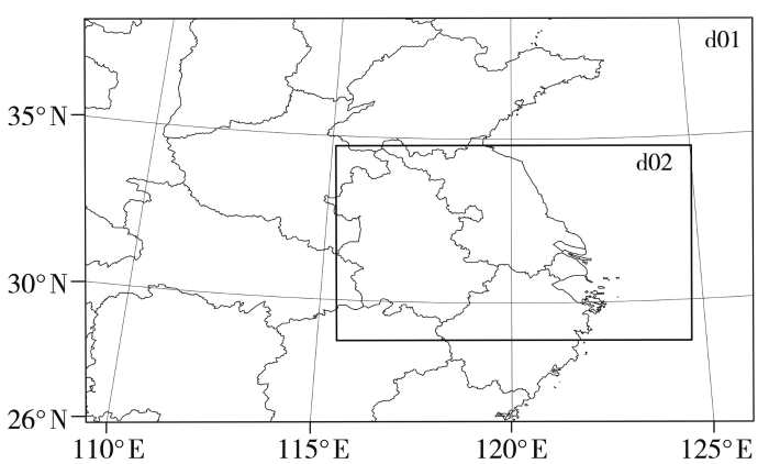
试验采用WRF3.8版本(Weather Research and Forecasting Model version 3.8),进行两重嵌套(图1),模拟区域中心为117.50°E、32.50°N,内外层水平分辨率分别为2、6 km,格点数分别是451×331、283×229,垂直方向为不等距30层,模式顶层气压为50 hPa,积分时间为2016年7月29日08:00—20:00,共12 h,积分时间步长36 s,每6 min输出一次结果。对于其他主要物理方案,内外层设置一致:关闭积云对流方案,采用WDM6微物理方案、Dudhia短波辐射方案、RRTMG长波辐射方案和Noah陆面过程方案。基于上述模式设置,选择YSU和ACM2两个边界层方案进行试验。
图1
1.2 边界层方案简介
式中:k为冯卡曼常数,取值0.4;ws(m·s-1)为混合层速度尺度;
ACM2方案是非局地向上混合和局地向下混合的不对称对流方案,通过计算总的混合速率来预报物理量的变化,其Km、Kt在混合层内计算公式(Pleim, 2007)如下:
式中:
式中:
表1 两个方案试验设置及命名
Tab.1
| 试验名称 | 试验设置 | 试验名称 | 试验设置 |
|---|---|---|---|
| YSU10 | p=1.00 | ACM10 | p=1.00 |
| YSU15 | p=1.50 | ACM15 | p=1.50 |
| YSU20 | p=2.00(模式默认值) | ACM20 | p=2.00(模式默认值) |
| YSU25 | p=2.50 | ACM25 | p=2.50 |
| YSU30 | p=3.00 | ACM30 | p=3.00 |
1.3 定量评估方法
为定量评估模拟结果,采用FSS(Fractions Skill Score)评分方法(Roberts and Lean, 2008),该评分利用方差技巧,通过计算格点上雷达反射率的区域命中率来评估模式模拟性能,是使用较为普遍的空间邻域检验方法,但需要首先确定评分阈值和影响邻域窗,评分阈值越小,邻域窗越大,评分越高。其计算公式如下:
式中:
2 个例简介
2016年7月25—30日,副高控制下上海及其附近地区连续数天发生午后强对流,南通站雷达观测(图2)显示,7月29日13:00左右,在江苏东南部和上海地区有对流触发,其最大组合反射率超过45 dBZ,14:00—15:00对流发展强盛,上海地区对流范围扩大,强度增强并朝西南方向移动,而江苏东南部的对流减弱,16:00对流消散。上海宝山站探空数据(图略)显示,29日08:00该地大气呈现上干冷下暖湿结构,对流有效位能(Convective Available Potential Energy, CAPE)为3 526.8 J·kg-1,说明该区不稳定能量较高;到14:00,CAPE增加到3 781.5 J·kg-1,对流抑制能量(Convective Inhibition, CIN)减小,同时700 hPa高度以下垂直风切变明显增强,为对流触发提供了较好的动力和热力条件。环流形势(图略)分析表明,29日08:00,上海及其附近地区500 hPa高度为平直的西风,850 hPa高度为偏西风,无明显天气系统影响。故认为这次对流过程是非系统性的局地热对流。
图2

图2
2016年7月29日南通站雷达组合反射率演变(单位:dBZ)
Fig.2
Evolution of radar composite reflectivity at Nantong station on 29 July 2016(Unit: dBZ)
此外,选取2013年8月16日发生在南京地区的一次热对流过程进行相似个例验证,该过程同为副高控制下的局地过程,无明显的大尺度动力特征,生命史只有2~3 h。
3 结果与分析
3.1 雷达反射率的发展演变
对于局地短时强对流,雷达反射率能给出较为及时且直观的时空信息,图3是不同垂直混合强度下YSU方案模拟的2016年7月29日13:00—16:00雷达组合反射率发展演变。可以看出,YSU10和YSU15试验对流触发时间均为14:00,15:00—16:00对流发展强盛,较观测晚1 h左右,对流的强度比观测弱,范围比观测小;而YSU20、YSU25和YSU30试验都能准确模拟出对流13:00触发、14:00—15:00发展强盛和16:00消散的演变过程,强度和范围与观测接近。ACM2方案的所有试验模拟的对流触发时间均晚于观测,且模拟的对流强度和范围均比观测小(图4),其中ACM10和ACM15试验对流触发时间为15:00前后,16:00—17:00发展强盛,较观测晚约2 h;ACM20、ACM25和ACM30试验对流触发时间在14:30左右,15:00—16:00发展强盛,较观测晚约1 h。此外,两个方案都能很好地模拟出对流位置。可见,减弱垂直混合会更早地触发对流,并且获得更大的对流范围和更强的对流强度,增强垂直混合则相反。
图3
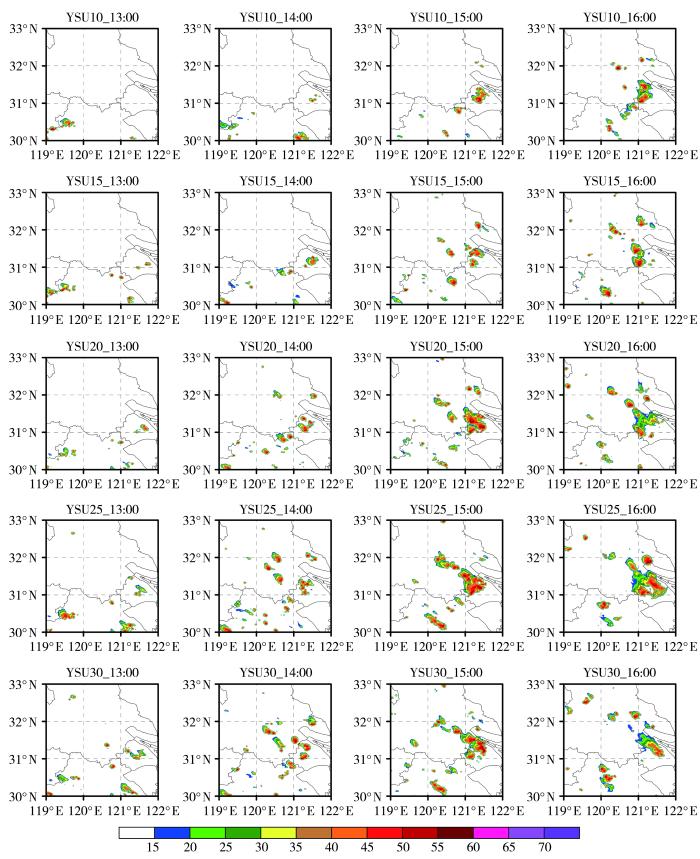
图3
不同垂直混合强度下YSU方案模拟的2016年7月29日雷达组合反射率演变(单位:dBZ)
Fig.3
Evolution of simulated radar composite reflectivity under different vertical mixing intensities of YSU scheme on 29 July 2016 (Unit: dBZ)
图4
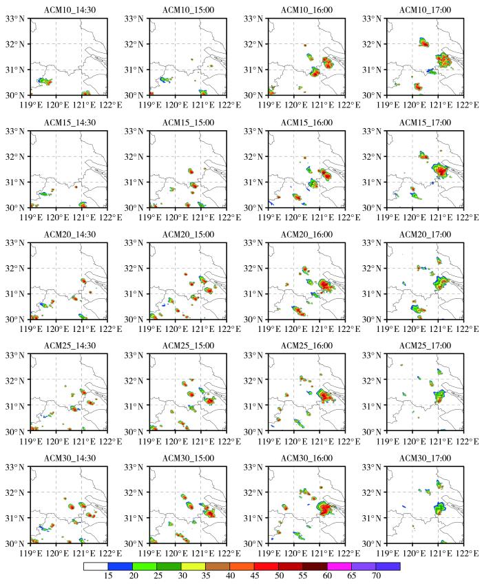
图4
不同垂直混合强度下ACM2方案模拟的2016年7月29日雷达组合反射率演变(单位:dBZ)
Fig.4
Evolution of simulated radar composite reflectivity under different vertical mixing intensities of ACM2 scheme on 29 July 2016 (Unit: dBZ)
为定量评估两方案不同垂直混合强度下的模拟效果,将YSU方案和ACM2方案模拟的对流发展阶段分别与雷达观测进行FSS定量评估(表2),发现13:00、14:00、15:00 YSU方案中评分最高的试验分别为YSU30、YSU25、YSU25,FSS值分别为0.144、0.480、0.275,13:00—15:00,YSU25和YSU30试验的FSS值整体高于YSU10和YSU15试验。14:30、15:00、16:00 ACM2方案中评分最高的试验均为ACM30试验,FSS值分别为0.303、0.403、0.307;14:30和15:00,ACM25评分略低于ACM30;17:00,ACM20评分最高(0.163),但在14:30和15:00 ACM20评分均低于ACM30和ACM25试验;ACM10和ACM15试验整体评分低于ACM30和ACM25试验。结合雷达组合反射率演变(图3、图4)分析可知,减弱垂直混合得到更接近观测的模拟结果,因为其能更准确地模拟对流触发和发展演变。此外,YSU25试验在对流发展演变及定量评估中均表现最优,因此认为该试验中垂直混合强度为局地热对流模拟的最佳混合强度。
表2 不同垂直混合强度下两种方案模拟的雷达组合反射率FSS值
Tab.2
| 试验名称 | 13:00 | 14:00 | 15:00 | 16:00 | 试验名称 | 14:30 | 15:00 | 16:00 | 17:00 |
|---|---|---|---|---|---|---|---|---|---|
| YSU10 | 0.000 | 0.000 | 0.170 | 0.099 | ACM10 | 0.000 | 0.032 | 0.284 | 0.103 |
| YSU15 | 0.000 | 0.072 | 0.176 | 0.006 | ACM15 | 0.000 | 0.135 | 0.196 | 0.118 |
| YSU20 | 0.000 | 0.371 | 0.205 | 0.044 | ACM20 | 0.073 | 0.273 | 0.236 | 0.163 |
| YSU25 | 0.003 | 0.480 | 0.275 | 0.054 | ACM25 | 0.211 | 0.337 | 0.221 | 0.013 |
| YSU30 | 0.144 | 0.336 | 0.175 | 0.056 | ACM30 | 0.303 | 0.403 | 0.307 | 0.007 |
注:评分阈值为35 dBZ,邻域窗大小为5×5个格点。
3.2 边界层演变
3.2.1 边界层高度
边界层内垂直混合强度能够通过边界层高度来反映,垂直混合越强(弱),边界层高度越高(低)(车军辉等,2021;Shin and Hong, 2011;Hu et al., 2010)。选取强对流区(121.0°E—121.5°E,31.0°N—31.5°N),对比两种方案模拟的区域平均边界层高度随时间变化(图5)。可以看到,随着参数p值减小,两种方案边界层高度都升高,说明垂直混合强度随参数p减小而增强,但ACM2方案模拟的边界层高度高于YSU方案,表明ACM2方案的垂直混合强度更强。YSU20、YSU25和YSU30(YSU10和YSU15)试验边界层高度在13:00(14:00)左右迅速降低,而ACM20、ACM25和ACM30(ACM10和ACM15)试验边界层高度在14:00(15:00)后开始迅速降低。边界层高度迅速降低的时间对应各实验对流触发时间,说明不同垂直混合强度对触发对流有重要贡献。
图5
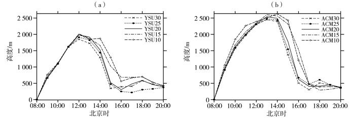
图5
不同垂直混合强度下YSU(a)和ACM2(b)方案模拟的2016年7月29日区域平均边界层高度随时间变化
Fig.5
The time series of simulated regional mean boundary layer height under different vertical mixing intensities of YSU (a) and ACM2 (b) schemes
3.2.2 边界层结构
图6为不同垂直混合强度下两方案模拟的2016年7月29日区域平均纬向风(u)、经向风(v)、位温(θ)及水汽混合比(q)的垂直廓线。YSU25和YSU30在14:00模拟出较大的风速和垂直风切变(风速或风向随高度变化较大),有利于对流触发和发展,15:00模拟的风速和垂直风切变减弱,对流开始减弱;YSU10和YSU15试验模拟的14:00风速和垂直风切变较小,15:00明显增大。ACM2方案中,ACM25和ACM30试验在14:30和16:00垂直风切变更大。上述结果表明,对流触发时减弱垂直混合可获得较大的边界层风速和垂直风切变,而对流旺盛时风速和垂直风切变减弱不利于对流维持和发展。
图6
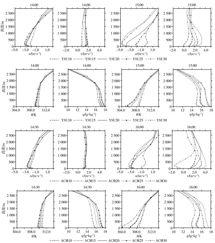
图6
不同垂直混合强度下两种方案模拟的2016年7月29日不同时刻区域平均纬向风(u)、经向风(v)、位温(θ)及水汽混合比(q)垂直廓线
(横坐标正负表示风向,向东和向北为正,向西和向南为负)
Fig.6
The vertical profile of simulated regional mean zonal wind (u), meridional wind (v), potential temperature (θ) and water vapor mixing ratio (q) at different time on 29 July 2016 under different vertical mixing intensities of two schemes
(The positive and negative on the horizontal axis indicate the wind direction, which are positive to the east and the north, and negative to the west and the south)
边界层内θ和q随高度变化梯度很小的区域称为混合层。14:00,YSU30模拟的混合层θ比YSU10低约1 K,YSU25和YSU30试验模拟的混合层q约18 g·kg-1,比YSU10试验多约1 g·kg-1;15:00,ACM30模拟的混合层θ也比ACM10低1 K左右,ACM25和ACM30试验模拟的混合层q约17.5 g·kg-1,较ACM10试验多约1.5 g·kg-1,表明减弱垂直混合使得混合层变湿冷,有利于不稳定能量累积。YSU25和YSU30试验在15:00、ACM25和ACM30试验在16:00混合层结构被明显破坏,θ和q明显减小;在近地面,YSU30和YSU25试验降温约3 K,ACM30试验降温约5 K;这几组试验在500~2 000 m高度q随高度增大,存在逆湿层,同时边界层上部由于水汽凝结释放潜热θ较高,而近地面由于降雨θ明显降低。而YSU10和YSU15试验在15:00、ACM10和ACM15试验在16:00处于对流发展时期,混合层q>17 g·kg-1,无明显变干和逆湿层,位温降低不明显。
3.3 能量演变
对流有效位能(CAPE)能够反映对流的发展潜势,对流抑制能量(CIN)则反映对流发展需要的能量下限(Wang et al., 2021;杨茜茜等, 2019)。由不同垂直混合强度下两种方案模拟的2016年7月29日区域平均CAPE和CIN随时间变化(图7)看出,29日08:00—11:00两方案的CIN值都快速降低,YSU方案在11:00—14:00、ACM2方案在11:00—15:00 CIN值均较低,最低时均不足10 J·kg-1,表明对流发展需要的下限能量非常低,容易发生对流。14:00前,YSU20、YSU25和YSU30试验模拟的CAPE值较大,14:00—16:00迅速降低,表明有较大的能量释放,其中YSU25试验释放能量超过1 600 J·kg-1,而YSU10和YSU15试验在14:00前CAPE值更低,16:00左右开始释放能量,释放能量不足1 000 J·kg-1,说明YSU25试验对流发展的时间早于YSU10和YSU15试验,且对流发展强度更强。ACM2方案中,ACM25和ACM30试验模拟的CAPE值更高,在14:30左右开始降低,14:30—17:00释放能量约1 200 J·kg-1,而ACM10试验模拟的CAPE值最低,且17:00左右开始降低,释放能量约600 J·kg-1,ACM15试验模拟的CAPE值变化与ACM10试验相似。这表明更强的垂直混合模拟的不稳定能量偏低,不利于更早触发对流,且释放能量较少,不利于对流强烈发展。
图7
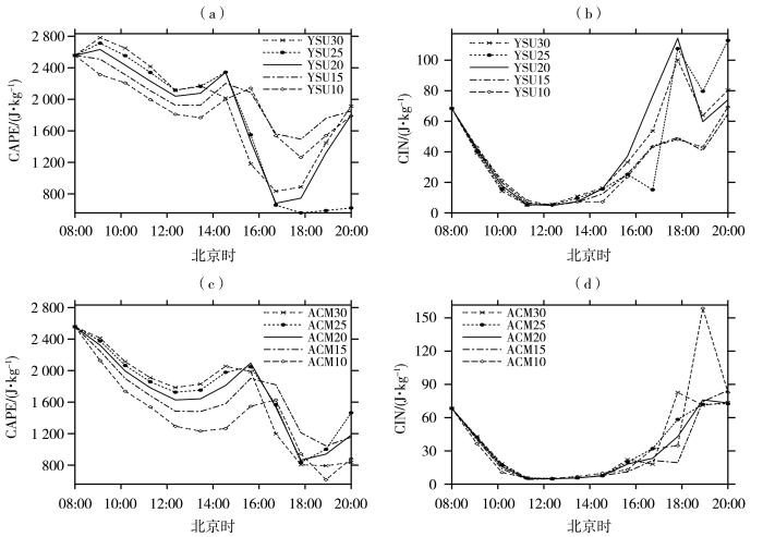
图7
不同垂直混合强度下YSU(a、b)和ACM2(c、d)方案模拟的2016年7月29日区域平均CAPE(a、c)和CIN(b、d)随时间变化
Fig.7
The times series of simulated regional mean CAPE (a, c) and CIN (b, d) on 29 July 2016 under different vertical mixing intensities of YSU (a, b) and ACM2 (c, d) schemes
4 相似个例验证
选取2013年8月16日副高控制下在南京地区发生的一次午后热对流过程对上述结论进行验证,并使用南京站多普勒天气雷达观测资料分析模拟结果。图8是观测和不同垂直混合强度下两种方案模拟的2013年8月16日南京地区雷达组合反射率演变。观测表明,16日13:00左右,在南京南边出现两个对流单体,其中偏南的对流单体持续发展,在14:00左右发展成熟,而偏北的对流单体消散,同时在南京北部出现新的对流,到15:00,偏南的对流单体消散,南京市的对流发展为东北—西南向的条状。模拟结果表明,YSU方案在13:30触发对流,比观测晚约半小时,而ACM2方案则在14:30触发对流,比观测晚一个半小时。两个方案中,YSU10和ACM10完全没有模拟出对流的触发(图略),YSU15在14:00、ACM15在15:00模拟出对流触发,分别比YSU20和ACM20试验迟,YSU25、YSU30、ACM25、ACM30均模拟出了几个对流单体的发展演变,且成熟阶段对流体强度和落区都更接近观测。
图8
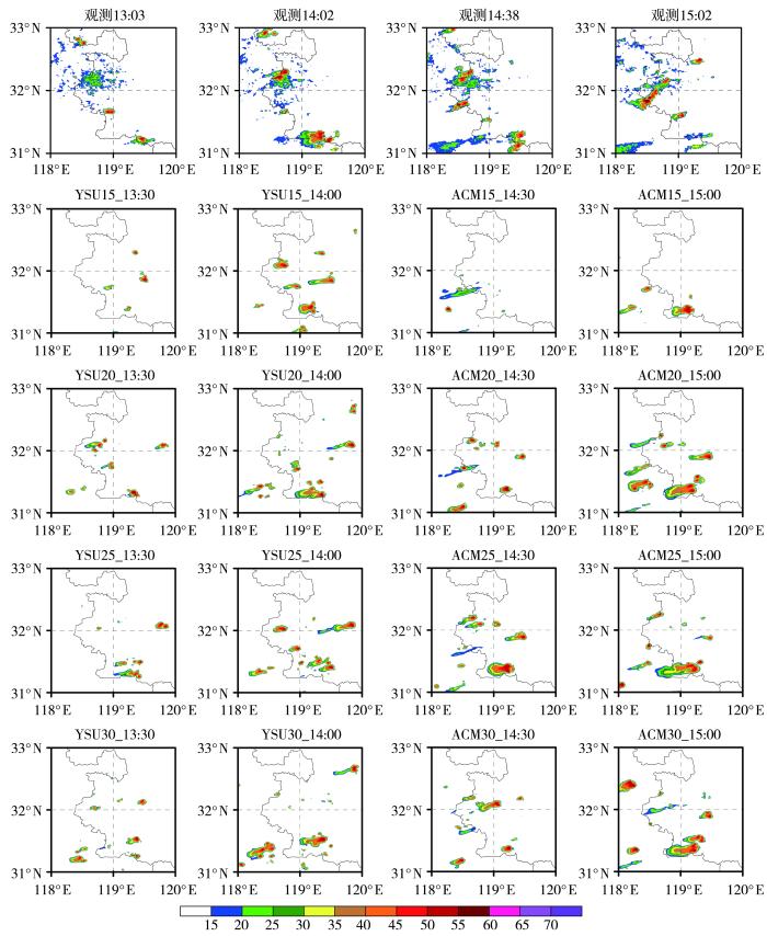
图8
观测和不同垂直混合强度下两种方案模拟的2013年8月16日南京地区雷达组合反射率演变(单位:dBZ)
Fig.8
Evolution of observed and simulated radar composite reflectivity at Nanjing on 16 August 2013 under different vertical mixing intensities of two schemes (Unit: dBZ)
此外,对该热对流过程强对流区域(119.0°E—119.5°E,31.0°N—31.5°N)的边界层高度、边界层结构和能量演变(图略)分析也表明,减弱垂直混合强度使得边界层内更湿冷,触发前边界层内风速和垂直风切变更大,模拟出更大的CAPE值而更早触发对流。
综上所述,在副高控制下局地热对流的数值模拟中,无论是YSU还是ACM2边界层方案,模式默认的垂直混合强度都不能很好地模拟局地热对流的发展演变过程,通过调整两方案中参数p值为2.50或3.00,减弱湍流的垂直输送,均能够改善模拟结果。
5 结论
针对弱环境场下局地对流难以准确预报,调整边界层湍流混合强度能否改善对流触发这一问题,利用中尺度模式WRF中的YSU和ACM2边界层方案,模拟了2016年7月29日长江下游地区发生的一次局地热对流过程,并通过相似个例检验,探究两种边界层方案(YSU和ACM2)中不同垂直混合强度对局地热对流数值模拟的影响,结果如下:
无论是YSU方案还是ACM2方案,模式默认的垂直混合强度都无法准确模拟局地热对流的触发和演变,减弱垂直混合强度能够改善对流触发时间和发展演变。YSU方案中,YSU25、YSU30试验模拟的对流发展演变和强度更接近观测。与YSU方案相比,ACM2方案对流触发较晚。FSS定量评估表明,YSU25和YSU30、ACM25和ACM30模拟结果较好,其中YSU25试验模拟效果最佳。即对于弱环境场局地热对流,采用模式默认值模拟的垂直混合强度过强,减弱垂直混合强度可以在一定程度上提高模拟精度。进一步分析表明,减弱垂直混合强度后边界层高度明显降低,其中YSU方案模拟值随时间变化与观测的对流时间演变较一致;ACM2方案边界层高度高于YSU方案,表明其垂直混合强度更强,导致对流发展更迟。在对流触发时,减弱垂直混合强度使得边界层内更湿冷,风速和垂直风切变增大,同时模拟出更大的CAPE值而有利于更早触发对流,对流强度也更强。
上述结果基于两个个例,是否适用于类似背景下其他局地热对流模拟还需要更多个例验证,但本研究提供的问题线索可为后续深入研究提供参考。
致谢
本研究工作得到兰州大学超算平台支持。
参考文献
西太平洋副热带高压控制下湖南一次短时强降水成因分析
[J].
在天气预报业务中,发生在西太平洋副热带高压控制下的短时强降水容易出现漏报。为加深对西太平洋副热带高压控制下湖南短时强降水的认识,探究其成因和触发机制,本文利用地面自动站、多普勒天气雷达观测资料及FY-2F云顶亮温、NCEP再分析资料等,针对2018年9月6日一次西太平洋副热带高压控制下的湖南短时强降水成因开展研究。结果表明:在强盛的西太平洋副热带高压脊区内,丰沛的水汽、较强的不稳定能量及一定的抬升条件可触发短时强降水天气。正午前,受弱冷空气侵入影响,低层切变配合地面中尺度辐合线引起近地面动力抬升,从而触发对流性降水;午后,受太阳辐射影响,地面气温达到对流触发温度,从而触发热对流。正涡度区及低层辐合区在降水发生后都向上延伸,有利于垂直上升运动的维持,但较典型汛期强降水过程的动力条件明显偏弱。环境风及其垂直风切变小,且雷暴单体移动缓慢,有利于强降水在同一地区长时间维持。
不同方法对青海 2020 年强降水模式产品预报性能的检验对比
[J].基于多模式降水格点预报资料、青海省气象站实况资料及多源融合降水格点分析产品,针对青海省2020年7—8月强降水天气个例,采用TS(threat score)评分等传统检验方法和FSS(fraction skill score)评分及MODE(method of object-based diagnostic evaluation)空间检验方法,对比检验各模式在青海强降水中的预报性能。结果表明:(1)小雨及以上量级,欧洲中期天气预报中心(ECMWF)和美国国家环境预报中心(NCEP)全球模式、中国气象局全球同化预报系统(CMA-GFS)及GRAPES区域中尺度数值预报系统(GRAPES-Meso)的传统TS评分均较高且预报能力相差不大,但不同检验方法下评分最高的模式略有不同;(2)中雨及以上量级,各模式预报较观测普遍偏西,且传统TS评分差异较为明显,但不同检验方法下模式评分优劣表现较为一致;(3)大雨及以上量级,各模式预报较观测普遍偏北,且预报能力较差,传统TS评分为0,FSS评分有效提高了模式差异性的评估能力,MODE方法则给出了预报和观测对象属性的具体表现,但对检验参数的选取较为敏感。
大气边界层数值模拟研究与未来展望
[J].大气边界层作为连接下垫面和自由大气的重要桥梁,不仅影响局地的各种天气过程的发展和演变,而且在区域和全球的天气和气候变化中也扮演着关键角色。鉴于大气边界层自身的复杂性,对其数值模拟一直以来都是大气数值模拟研究中的热点和难点。通过归纳近几十年来大气边界层数值模式发展经历的3个阶段,梳理了干旱半干旱区、青藏高原地区和城市复杂下垫面3个陆地气候关键区边界层过程,以及海洋上特殊的台风边界层数值模拟研究取得的重要进展;总结出当前大气边界层数值模拟研究所面临的5个亟待解决的关键科学问题:云与边界层相互作用、边界层参数化、模式分辨率、边界层资料同化以及边界层发展机制。并明确了该领域未来需要在加强不同类型大气边界层过程的认识、边界层底和顶界面交换过程的理解、特殊地区边界层发展机制的解释、边界层参数化方案的改进、大涡模拟在边界层模拟中优势的充分发挥等5个方面开展重点研究,以期能为今后更系统地开展大气边界层数值模拟及相关研究提供参考依据。
边界层参数化方案对不同性质降水模拟的影响
[J].利用MM5模式的4种边界层方案(ETA方案\, MRF方案\, Blackadar方案\, Gayno\|Seman方案), 对2008年9月22~27日发生在四川盆地先是对流性, 后来是稳定性的暴雨过程进行了该4种不同边界层方案的数值模拟比较试验。整体而言, ETA方案对雨带的预报能力较差, 但对对流性降水有一定的预报能力; MRF方案对雨带(特别是稳定性降水)的预报能力相对最强; Blackadar方案对后24 h强降水最具能力, 且对对流性和稳定性降水的预报能力没有太大差别; Gayno-Seman方案对后24 h强降水预报能力较差。边界层对物理量场的影响随时间增大。在预报积分的前10 h以内, 各方案的涡度、 相对湿度、 垂直速度等物理量预报几乎无异; 积分10~24 h, 它们的量值间出现差异; 24 h后, 不同方案的预报不仅量值上有差异, 甚至变化趋势都不尽相同。高度场受边界层的影响最小, 受边界层方案影响最大的是U场, V场受边界层的影响呈高度和时间的分段函数, 湿度场受到的影响有明显的时间滞后性特征。对于温度场而言, 600 hPa似乎是温度场受边界层影响的一个拐点, 边界层影响在通过600 hPa后改变了影响规律。
The influence of PBL parameterization on the practical predictability of convection initiation during the Mesoscale Predictability Experiment (MPEX)
[J].This study evaluates the influence of planetary boundary layer parameterization on short-range (0–15 h) convection initiation (CI) forecasts within convection-allowing ensembles that utilize subsynoptic-scale observations collected during the Mesoscale Predictability Experiment. Three cases, 19–20 May, 31 May–1 June, and 8–9 June 2013, are considered, each characterized by a different large-scale flow pattern. An object-based method is used to verify and analyze CI forecasts. Local mixing parameterizations have, relative to nonlocal mixing parameterizations, higher probabilities of detection but also higher false alarm ratios, such that the ensemble mean forecast skill only subtly varied between parameterizations considered. Temporal error distributions associated with matched events are approximately normal around a zero mean, suggesting little systematic timing bias. Spatial error distributions are skewed, with average mean (median) distance errors of approximately 44 km (28 km). Matched event cumulative distribution functions suggest limited forecast skill increases beyond temporal and spatial thresholds of 1 h and 100 km, respectively. Forecast skill variation is greatest between cases with smaller variation between PBL parameterizations or between individual ensemble members for a given case, implying greatest control on CI forecast skill by larger-scale features than PBL parameterization. In agreement with previous studies, local mixing parameterizations tend to produce simulated boundary layers that are too shallow, cool, and moist, while nonlocal mixing parameterizations tend to be deeper, warmer, and drier. Forecasts poorly resolve strong capping inversions across all parameterizations, which is hypothesized to result primarily from implicit numerical diffusion associated with the default finite-differencing formulation for vertical advection used herein.
A review of planetary boundary layer parameterization schemes and their sensitivity in simulating Southeastern U.S. cold season severe weather environments
[J].The representation of turbulent mixing within the lower troposphere is needed to accurately portray the vertical thermodynamic and kinematic profiles of the atmosphere in mesoscale model forecasts. For mesoscale models, turbulence is mostly a subgrid-scale process, but its presence in the planetary boundary layer (PBL) can directly modulate a simulation’s depiction of mass fields relevant for forecast problems. The primary goal of this work is to review the various parameterization schemes that the Weather Research and Forecasting Model employs in its depiction of turbulent mixing (PBL schemes) in general, and is followed by an application to a severe weather environment. Each scheme represents mixing on a local and/or nonlocal basis. Local schemes only consider immediately adjacent vertical levels in the model, whereas nonlocal schemes can consider a deeper layer covering multiple levels in representing the effects of vertical mixing through the PBL. As an application, a pair of cold season severe weather events that occurred in the southeastern United States are examined. Such cases highlight the ambiguities of classically defined PBL schemes in a cold season severe weather environment, though characteristics of the PBL schemes are apparent in this case. Low-level lapse rates and storm-relative helicity are typically steeper and slightly smaller for nonlocal than local schemes, respectively. Nonlocal mixing is necessary to more accurately forecast the lower-tropospheric lapse rates within the warm sector of these events. While all schemes yield overestimations of mixed-layer convective available potential energy (MLCAPE), nonlocal schemes more strongly overestimate MLCAPE than do local schemes.
Processes associated with convection initiation in the North American Mesoscale Forecast System, version 3 (NAMv3)
[J].In support of the Next Generation Global Prediction System (NGGPS) project, processes leading to convection initiation in the North American Mesoscale Forecast System, version 3 (NAMv3) are explored. Two severe weather outbreaks—occurring over the southeastern United States on 28 April 2014 and the central Great Plains on 6 May 2015—are forecast retrospectively using the NAMv3 CONUS (4 km) and Fire Weather (1.33 km) nests, each with 5-min output. Points of convection initiation are identified, and patterns leading to convection initiation in the model forecasts are determined. Results indicate that in the 30 min preceding convection initiation at a grid point, upward motion at low levels of the atmosphere enables a parcel to rise to its level of free convection, above which it is accelerated by the buoyancy force. A moist absolutely unstable layer (MAUL) typically is produced at the top of the updraft. However, when strong updrafts are collocated with large vertical gradients of potential temperature and moisture, noisy vertical profiles of temperature, moisture, and hydrometeor concentration develop beneath the rising MAUL. The noisy profiles found in this study are qualitatively similar to those that resulted in NAMv3 failures during simulations of Hurricane Joaquin in 2015. The CM1 cloud model is used to reproduce these noisy profiles, and results indicate that the noise can be mitigated by including explicit vertical diffusion in the model. Left unchecked, the noisy profiles are shown to impact convective storm features such as cold pools, precipitation, updraft helicity intensity and tracks, and the initiation of spurious convection.
Verification of convection-allowing WRF model forecasts of the planetary boundary layer using sounding observations
[J].This study evaluates forecasts of thermodynamic variables from five convection-allowing configurations of the Weather Research and Forecasting Model (WRF) with the Advanced Research core (WRF-ARW). The forecasts vary only in their planetary boundary layer (PBL) scheme, including three “local” schemes [Mellor–Yamada–Janjić (MYJ), quasi-normal scale elimination (QNSE), and Mellor–Yamada–Nakanishi–Niino (MYNN)] and two schemes that include “nonlocal” mixing [the asymmetric cloud model version 2 (ACM2) and the Yonei University (YSU) scheme]. The forecasts are compared to springtime radiosonde observations upstream from deep convection to gain a better understanding of the thermodynamic characteristics of these PBL schemes in this regime. The morning PBLs are all too cool and dry despite having little bias in PBL depth (except for YSU). In the evening, the local schemes produce shallower PBLs that are often too shallow and too moist compared to nonlocal schemes. However, MYNN is nearly unbiased in PBL depth, moisture, and potential temperature, which is comparable to the background North American Mesoscale model (NAM) forecasts. This result gives confidence in the use of the MYNN scheme in convection-allowing configurations of WRF-ARW to alleviate the typical cool, moist bias of the MYJ scheme in convective boundary layers upstream from convection. The morning cool and dry biases lead to an underprediction of mixed-layer CAPE (MLCAPE) and an overprediction of mixed-layer convective inhibition (MLCIN) at that time in all schemes. MLCAPE and MLCIN forecasts improve in the evening, with MYJ, QNSE, and MYNN having small mean errors, but ACM2 and YSU having a somewhat low bias. Strong observed capping inversions tend to be associated with an underprediction of MLCIN in the evening, as the model profiles are too smooth. MLCAPE tends to be overpredicted (underpredicted) by MYJ and QNSE (MYNN, ACM2, and YSU) when the observed MLCAPE is relatively small (large).
Convection initiation and growth at the coast of South China. Part I: effect of the marine boundary layer jet
[J].Convection initiation (CI) and the subsequent upscale convective growth (UCG) at the coast of South China in a warm-sector heavy rainfall event are shown to be closely linked to a varying marine boundary layer jet (MBLJ) over the northern South China Sea (NSCS). To elucidate the dynamic and thermodynamic roles of the MBLJ in CI and UCG, we conducted and analyzed convection-permitting numerical simulations and observations. Compared to radar observations, the simulations captured CI locations and the following southwest–northeast-oriented convection development. The nocturnal MBLJ peaks at 950 hPa and significantly intensifies with turning from southwesterly to nearly southerly by inertial oscillation. The strengthened MBLJ promotes mesoscale ascent on its northwestern edge and terminus where enhanced convergence zones occur. Located directly downstream of the MBLJ, the coastal CI and UCG are dynamically supported by mesoscale ascent. From a thermodynamic perspective, a warm moist tongue over the NSCS is strengthened by the MBLJ-driven mesoscale ascent as well as by a high sea surface temperature. The warm moist tongue farther extends northeastward by horizontal transport and arrives at the coast where CI and UCG occur. Near the CI location, rapid development of a low-level saturated layer is mainly attributed to the mesoscale ascent and low-level moistening associated with the MBLJ. In addition, subsequent CI happens on either side of the original CI along the coast due to the delay of low-level moistening, which partly contributes to linear convective growth. Furthermore, ensemble simulations confirmed that a stronger MBLJ is more favorable to CI and UCG near the coast.
Seasonal dependence of WRF model biases and sensitivity to PBL schemes over Europe
[J].
A new vertical diffusion package with an explicit treatment of entrainment processes
[J].This paper proposes a revised vertical diffusion package with a nonlocal turbulent mixing coefficient in the planetary boundary layer (PBL). Based on the study of Noh et al. and accumulated results of the behavior of the Hong and Pan algorithm, a revised vertical diffusion algorithm that is suitable for weather forecasting and climate prediction models is developed. The major ingredient of the revision is the inclusion of an explicit treatment of entrainment processes at the top of the PBL. The new diffusion package is called the Yonsei University PBL (YSU PBL). In a one-dimensional offline test framework, the revised scheme is found to improve several features compared with the Hong and Pan implementation. The YSU PBL increases boundary layer mixing in the thermally induced free convection regime and decreases it in the mechanically induced forced convection regime, which alleviates the well-known problems in the Medium-Range Forecast (MRF) PBL. Excessive mixing in the mixed layer in the presence of strong winds is resolved. Overly rapid growth of the PBL in the case of the Hong and Pan is also rectified. The scheme has been successfully implemented in the Weather Research and Forecast model producing a more realistic structure of the PBL and its development. In a case study of a frontal tornado outbreak, it is found that some systematic biases of the large-scale features such as an afternoon cold bias at 850 hPa in the MRF PBL are resolved. Consequently, the new scheme does a better job in reproducing the convective inhibition. Because the convective inhibition is accurately predicted, widespread light precipitation ahead of a front, in the case of the MRF PBL, is reduced. In the frontal region, the YSU PBL scheme improves some characteristics, such as a double line of intense convection. This is because the boundary layer from the YSU PBL scheme remains less diluted by entrainment leaving more fuel for severe convection when the front triggers it.
Evaluation of three planetary boundary layer schemes in the WRF model
[J].Accurate depiction of meteorological conditions, especially within the planetary boundary layer (PBL), is important for air pollution modeling, and PBL parameterization schemes play a critical role in simulating the boundary layer. This study examines the sensitivity of the performance of the Weather Research and Forecast (WRF) model to the use of three different PBL schemes [Mellor–Yamada–Janjic (MYJ), Yonsei University (YSU), and the asymmetric convective model, version 2 (ACM2)]. Comparison of surface and boundary layer observations with 92 sets of daily, 36-h high-resolution WRF simulations with different schemes over Texas in July–September 2005 shows that the simulations with the YSU and ACM2 schemes give much less bias than with the MYJ scheme. Simulations with the MYJ scheme, the only local closure scheme of the three, produced the coldest and moistest biases in the PBL. The differences among the schemes are found to be due predominantly to differences in vertical mixing strength and entrainment of air from above the PBL. A sensitivity experiment with the ACM2 scheme confirms this diagnosis.
Mesoscale meteorology in midlatitudes
[M].
Evaluation of planetary boundary layer scheme sensitivities for the purpose of parameter estimation
[J].Meteorological model errors caused by imperfect parameterizations generally cannot be overcome simply by optimizing initial and boundary conditions. However, advanced data assimilation methods are capable of extracting significant information about parameterization behavior from the observations, and thus can be used to estimate model parameters while they adjust the model state. Such parameters should be identifiable, meaning that they must have a detectible impact on observable aspects of the model behavior, their individual impacts should be a monotonic function of the parameter values, and the various impacts should be clearly distinguishable from each other.
Improvement of the K-profile model for the planetary boundary layer based on large eddy simulation data
[J].
A combined local and nonlocal closure model for the atmospheric boundary layer. Part I: model description and testing
[J].The modeling of the atmospheric boundary layer during convective conditions has long been a major source of uncertainty in the numerical modeling of meteorological conditions and air quality. Much of the difficulty stems from the large range of turbulent scales that are effective in the convective boundary layer (CBL). Both small-scale turbulence that is subgrid in most mesoscale grid models and large-scale turbulence extending to the depth of the CBL are important for the vertical transport of atmospheric properties and chemical species. Eddy diffusion schemes assume that all of the turbulence is subgrid and therefore cannot realistically simulate convective conditions. Simple nonlocal closure PBL models, such as the Blackadar convective model that has been a mainstay PBL option in the fifth-generation Pennsylvania State University–National Center for Atmospheric Research Mesoscale Model (MM5) for many years and the original asymmetric convective model (ACM), also an option in MM5, represent large-scale transport driven by convective plumes but neglect small-scale, subgrid turbulent mixing. A new version of the ACM (ACM2) has been developed that includes the nonlocal scheme of the original ACM combined with an eddy diffusion scheme. Thus, the ACM2 is able to represent both the supergrid- and subgrid-scale components of turbulent transport in the convective boundary layer. Testing the ACM2 in one-dimensional form and comparing it with large-eddy simulations and field data from the 1999 Cooperative Atmosphere–Surface Exchange Study demonstrates that the new scheme accurately simulates PBL heights, profiles of fluxes and mean quantities, and surface-level values. The ACM2 performs equally well for both meteorological parameters (e.g., potential temperature, moisture variables, and winds) and trace chemical concentrations, which is an advantage over eddy diffusion models that include a nonlocal term in the form of a gradient adjustment.
Scale-selective verification of rainfall accumulations from high-resolution forecasts of convective events
[J].The development of NWP models with grid spacing down to ∼1 km should produce more realistic forecasts of convective storms. However, greater realism does not necessarily mean more accurate precipitation forecasts. The rapid growth of errors on small scales in conjunction with preexisting errors on larger scales may limit the usefulness of such models. The purpose of this paper is to examine whether improved model resolution alone is able to produce more skillful precipitation forecasts on useful scales, and how the skill varies with spatial scale. A verification method will be described in which skill is determined from a comparison of rainfall forecasts with radar using fractional coverage over different sized areas. The Met Office Unified Model was run with grid spacings of 12, 4, and 1 km for 10 days in which convection occurred during the summers of 2003 and 2004. All forecasts were run from 12-km initial states for a clean comparison. The results show that the 1-km model was the most skillful over all but the smallest scales (approximately <10–15 km). A measure of acceptable skill was defined; this was attained by the 1-km model at scales around 40–70 km, some 10–20 km less than that of the 12-km model. The biggest improvement occurred for heavier, more localized rain, despite it being more difficult to predict. The 4-km model did not improve much on the 12-km model because of the difficulties of representing convection at that resolution, which was accentuated by the spinup from 12-km fields.
Intercomparison of planetary boundary layer parametrizations in the WRF model for a single day from CASES-99
[J].
An introduction to boundary layer meteorology
[M].
High-resolution simulation of an extreme heavy rainfall event in Shanghai using the weather research and forecasting model: sensitivity to planetary boundary layer parameterization
[J].
Analysis of the role of the planetary boundary layer schemes during a severe convective storm
[J].. The role played by planetary boundary layer (PBL) in the development and evolution of a severe convective storm is studied by means of meso-scale modeling and surface and upper air observations. The severe convective precipitation event that occurred on 14 September 1999 in the northeast of the Iberian Peninsula was simulated by means of the mesoscale model MM5 (version 3) using three different PBL schemes. The numerical results show a large impact of the PBL schemes on the precipitation fields associated to the convective storm. The schemes are based on different physical assumptions: the nonlocal first order Medium-Range Forecast (MRF) and Blackadar (BLA) scheme and the local, one-and-a-half order ETA scheme. Surface and radar observations are used to validate the model results. The comparison focuses on three aspects: the evolution, the spatial distribution and the 24-h accumulated precipitation. The comparison with rain gauge observations shows that the MRF, BLA and ETA schemes predicted most of the precipitation during the morning, whereas the rain gauge stations recorded rainfall during the evening. The evaluation performed with the radar data shows that all three numerical simulations produced a realistic spatial accumulated precipitation distribution. According to the quantity distribution, all three numerical simulations were able to predict precipitation quantities comparable to the rain gauge measurements. The MRF scheme predicted the largest average accumulated precipitation and the largest average precipitation rate, whereas the ETA scheme predicted the smallest accumulated precipitation and average precipitation rate. However, the ETA scheme yielded the highest extreme precipitation rates. The performance of the three schemes is analyzed in terms of the vertical distribution of potential temperature, specific humidity and conserved variables, like equivalent potential temperature and total water content. The MRF scheme showed more evidence of enhanced mixing than did the other schemes. Due to this process, more moisture was more efficiently transported to the free atmosphere. Consequently, the MRF scheme predicts more widespread precipitation. Furthermore, the enhanced mixing led to a less sharp capping inversion. However, the stronger inversion resulting from suppressed mixing processes in the case of the ETA scheme yielded higher values of convective available potential energy (CAPE) than did the other two schemes. Consequently, the more extreme precipitation rates are simulated by MM5 when the ETA scheme is used.\n
Evaluation of nonlocal and local planetary boundary layer schemes in the WRF model
[J].
Parametric and structural sensitivities of turbine-height wind speeds in the boundary layer parameterizations in the Weather Research and Forecasting model
[J].

